
On this page
Questions about your own assay?
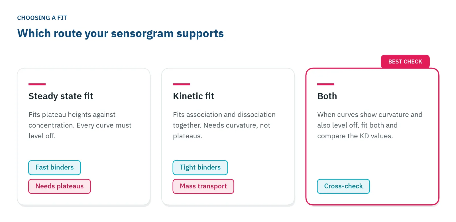
Ask a specialistA steady state affinity fit is only as good as its plateaus. If every curve flattens within the injection, fit the plateau responses against concentration. If the curves are still rising, the affinity will come out too weak: fit association and dissociation together instead, and check the two answers against each other when you can.
Two routes to the same KD
In label-free binding analysis, an analyte flows over an immobilized ligand. The signal rises while the sample is injected and falls when buffer returns, and this trace (the sensorgram) holds everything you need for an equilibrium dissociation constant (KD). You can get the KD in two ways, and each one works only when your data meet its assumptions.
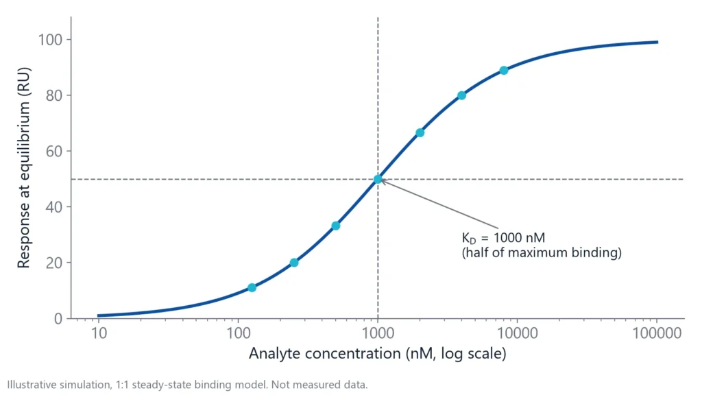
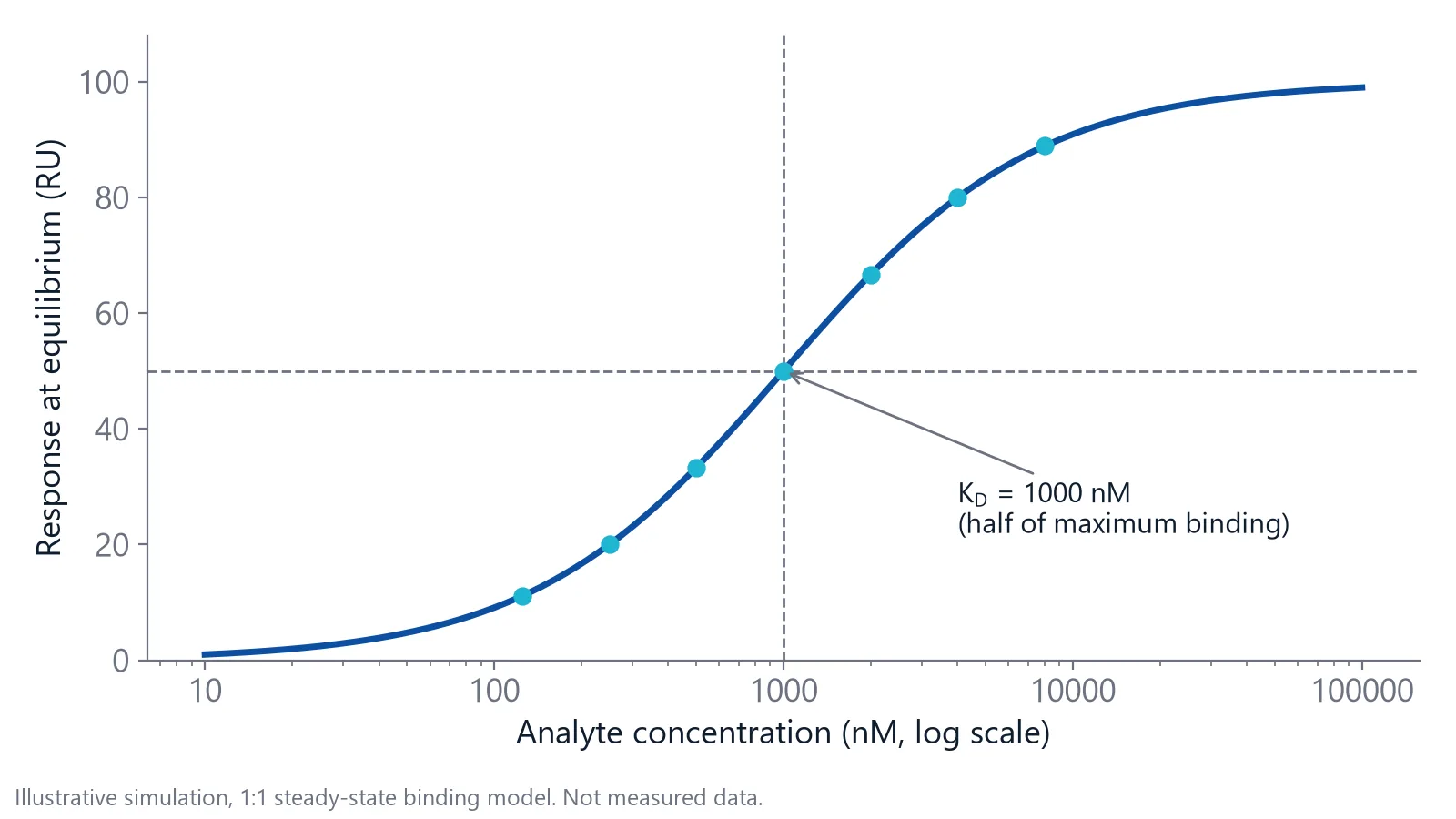
Steady state affinity uses only the plateau. When a curve levels off, as many complexes form as fall apart each second. The plateau height (Req) then depends on the number of binding sites, the analyte concentration and the KD [1]. Plot Req against concentration and fit a binding curve: at a concentration equal to the KD, half of the sites are occupied [1]. The one-to-one model is Req = Rmax x C / (KD + C), where C is the analyte concentration [1].
Kinetic analysis fits the curved parts of the sensorgram. It gives the association rate constant (kon, in 1/M/s) and the dissociation rate constant (koff, in 1/s), and KD is koff divided by kon [2]. A koff of 0.01 1/s means about 1% of the complexes fall apart every second.
The shape of your sensorgram decides which route your data can carry.
When should you use steady state affinity?
Use steady state affinity when binding is fast in both directions, so every curve flattens well within the injection and kon and koff are too fast to resolve. This is typical for weak binders, fragments and many small molecules. The plateaus are then the most reliable part of the data, and a kinetic fit has little curvature to work with [2,3].
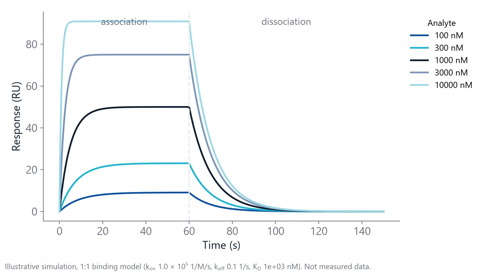
Spread the concentrations so the plateaus cover about 10% to 90% of saturation, roughly 0.1 to 10 times the expected KD [1]. Reaching 90% of the maximum response already takes about 10 times the KD [1]. Going much higher does not help: above about 100 times the KD, curves often stop looking exponential and the bulk shift distorts them [1].
Tight binders rarely reach a plateau
The time to reach steady state depends mainly on koff, and it is longest at the lowest analyte concentration [1,4]. A complex that dissociates slowly can need hours of injection before the low concentrations level off.
Take a binder with a kon of 105 1/M/s and a koff of 10-4 1/s, so a KD of 1 nM. The curve approaches its plateau with a rate constant of kon times concentration plus koff [1]. At 1 nM analyte that is 2 x 10⁻⁴ 1/s, and reaching 95% of the plateau takes about 15,000 seconds. That is more than four hours of injection for one concentration.
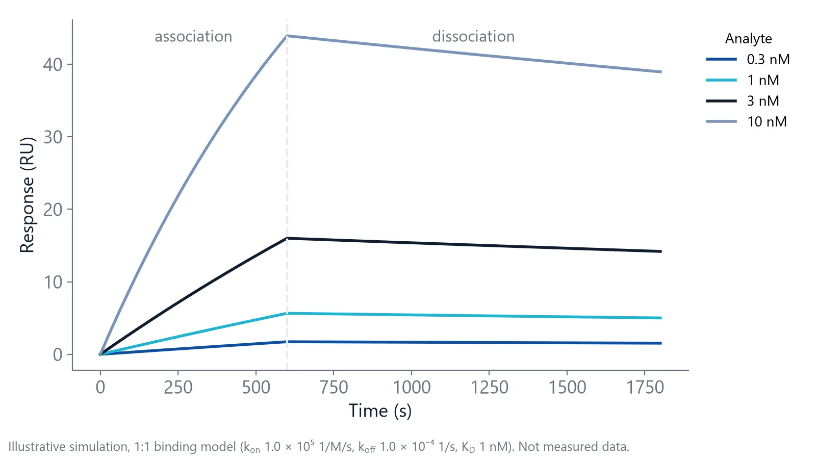
Fit those end points as if they were plateaus and the low concentrations fall furthest short, so the KD comes out too weak [4]. A survey of 100 binding studies found that most did not report a test for equilibration, and several reported affinities were incorrect [4]. Check that even the lowest concentration has reached its plateau, 95% or more by the equation above.
A kinetic fit does not need plateaus, only enough curvature in each curve [1]. For tight binders it is the better route, as long as the dissociation phase runs long enough to show a clear decay. Delta's application note on measuring tight binders shows a short and a long dissociation protocol for an antibody.
Check a steady state fit before you trust it
A steady state fit can look clean and still be wrong. Run these checks on your own data:
- Flat plateaus. Zoom in on the end of the injection at the lowest concentration. If it still rises, inject longer or switch to a kinetic fit.
- A curve that bends. If your highest concentration stays far below 10 times the fitted KD, the curve never flattens, and the fit has to guess where it would end. Treat that KD as an estimate.
- A plausible Rmax. Compare the fitted Rmax with what your ligand level and the analyte's mass predict. A much larger value means the fit extrapolated far beyond your data.
- Clean baselines. Subtract the reference channel and a buffer blank before you read plateaus. A buffer mismatch adds a step to every plateau [1].
Weak binders often fail the Rmax check. In a worked fragment example, even a nearly saturated fragment returned values that made no physical sense when Rmax and KD were both free. Fixing Rmax to an estimate, from a control compound scaled by molecular weight, gave a KD close to the concentration where the target was half saturated [5]. The authors treat such values as estimates for ranking, not exact constants [5]. For more on this group of analytes, see small molecule and peptide binding.
Kinetics shows what a KD hides
Two compounds with similar affinity can behave very differently. In a study of HIV-1 protease inhibitors, indinavir and saquinavir had similar inhibition constants, yet saquinavir dissociated far more slowly, with a half-life of about 6,500 seconds against 500 seconds [6]. A steady state KD alone would not separate them. When you need to know how long a complex lasts, as in antibody affinity and kinetics work, fit the kinetics.
Fit all concentrations together, so one kon and one koff must describe every curve. Then read the error of each parameter: a large standard error means the value can change a lot without making the fit worse, so it is not reliable [2].
Mass transport is the classic trap. When analyte binds faster than the flow can deliver it, the fitted kon and koff become unreliable, while the KD can still be recovered with a simpler affinity model [7].
Should steady state and kinetic KD values agree?
Yes. For a simple one-to-one interaction measured well, they should agree within about two-fold. One careful study reached that agreement between equilibrium and kinetic KD values and called it reasonable [4]. A larger gap means one of the two routes does not suit your data.
Variation between labs sets the scale. When 26 investigators measured 10 sulfonamides binding to carbonic anhydrase II, the errors in kon, koff and KD averaged 34, 24 and 37%, and the weakest and fastest binders varied most [8]. For a Fab fragment binding thyroxine analogs, kinetic, steady state and solution affinity analysis gave comparable values wherever more than one could be used [9].
When your two values disagree, check these causes:
- Steady state not reached: the steady state KD is the weaker of the two
- Mass transport: a plain one-to-one kinetic fit returns the wrong kon and koff, and its KD can drift too. Refit with a transport term or an affinity model; the KD from that fit should match the steady state value [7]
- A second binding site or a mixed surface: the dissociation is not a single exponential, so the kinetic fit shows systematic residuals while the steady state fit can still look clean
Agreement supports a KD but does not prove it [4]. Both routes use the analyte concentration you enter. If 90% of your analyte is inactive, the KD looks ten-fold weaker than it is [4], in both fits. Measure the active concentration of your analyte before you trust either number.
Questions researchers ask
Can I use single-cycle kinetics data for a steady state fit?
Only if each injection step reaches a flat plateau before the next one starts, which is rare for slow binders. Single-cycle runs use short steps with rising concentrations, so the response at the end of each step usually reflects time as much as affinity. For a steady state fit, use separate injections long enough to level off.
What is the offset in a steady state affinity model?
Many fitting programs add a constant offset to the binding curve. It absorbs a small response present at every concentration, often left over from imperfect referencing or a buffer mismatch. Check that it stays close to zero. A large offset means the plateaus contain more than specific binding, so fix the referencing before you fit again.
How many concentrations do I need for a steady state affinity fit?
Use at least five concentrations plus a buffer blank, spread around the expected KD with some below and some well above it. Repeat one concentration at the start and end of the series to check that the surface stays stable. If you do not know the KD yet, run a wide scouting series first.
Which KD should I report if I have both?
Report the one whose assumptions your data meet, and state the method, the concentration range and the contact time. If both are valid, report both and show the fits. Reviewers trust a KD more when they can see the plateaus or the residuals next to the number, not only a value in a table.
References
- Marquart JA. SPRpages – Getting a Feeling for the Curves. Handbook of Surface Plasmon Resonance. 2017. doi:10.1039/9781788010283-00106
- Real-Time Analysis of Biomolecular Interactions. Springer Japan. 2000. doi:10.1007/978-4-431-66970-8
- Apiyo DO. Biolayer Interferometry (Octet) for Label-free Biomolecular Interaction Sensing. Handbook of Surface Plasmon Resonance. 2017. doi:10.1039/9781788010283-00356
- Jarmoskaite I, AlSadhan I, Vaidyanathan PP et al.. How to measure and evaluate binding affinities. Elife. 2020. doi:10.7554/eLife.57264
- Karlsson R, Karlsson O, Belcher P. Fragment and Low Molecular Weight Compound Analysis. Handbook of Surface Plasmon Resonance. 2017. doi:10.1039/9781788010283-00255
- Markgren PO, Hämäläinen M, Danielson UH. Kinetic analysis of the interaction between HIV-1 protease and inhibitors using optical biosensor technology. Anal Biochem. 2000. doi:10.1006/abio.1999.4467
- Karlsson R. Affinity analysis of non-steady-state data obtained under mass transport limited conditions using BIAcore technology. J Mol Recognit. 1999. doi:10.1002/(SICI)1099-1352(199909/10)12:5<285::AID-JMR469>3.0.CO;2-Y
- Papalia GA, Leavitt S, Bynum MA et al.. Comparative analysis of 10 small molecules binding to carbonic anhydrase II by different investigators using Biacore technology. Anal Biochem. 2006. doi:10.1016/j.ab.2006.08.021
- Adamczyk M, Moore JA, Yu Z. Application of surface plasmon resonance toward studies of low-molecular-weight antigen-antibody binding interactions. Methods. 2000. doi:10.1006/meth.1999.0925
Keep reading
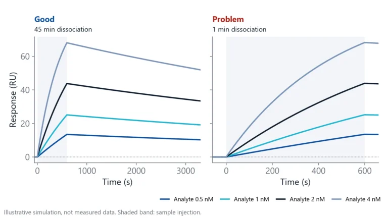 Biolayer interferometry vs SPR: which method fits your assayBoth methods measure binding label-free and in real time. The sample path, flow over a chip or a tip in a well, decides which one suits your hardest measurement.Applications
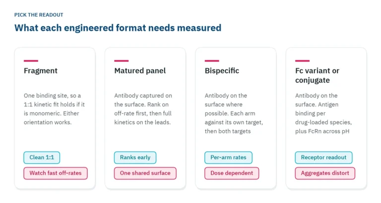 Antibody engineering: what binding data each format needsFragments, bispecifics, Fc variants and conjugates each need a different binding readout. Which parameter to measure, in which assay orientation, and why valency decides both.Applications
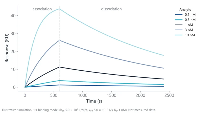 How to measure antibody binding kinetics: setup, rates and reportingA practical guide to antibody binding kinetics: which partner goes on the surface, how to set concentrations and times from the expected rates, how to check the fit and what to report.