
On this page
Questions about your own assay?
Ask a specialistA sensorgram shows binding at the sensor surface over time. Most misreadings happen because buffer jumps and drift look like binding, and slow transport distorts its shape. Here is how to read a sensorgram, in order: a flat baseline, an association that curves, a dissociation that returns to baseline. Then subtract the reference and a buffer blank before you fit.
How to read a sensorgram: what the curve shows
A label-free biosensor measures binding without a fluorescent or enzyme label. One partner, the ligand, is attached to the sensor surface. The other, the analyte, flows over it in solution. The sensorgram is the plot the instrument records: response on the y-axis, time on the x-axis.
Knowing how to read a sensorgram tells you whether your molecules bind, how fast they bind and how long they stay together. The response grows when mass collects at the surface and changes the refractive index there (how strongly the solution bends light). Many instruments report it in response units (RU); one RU is a refractive index change of 10-6 [1].
Surface plasmon resonance (SPR), biolayer interferometry (BLI), grating-coupled interferometry (GCI) and Nanophotonic Evanescent field Sensing (NES) all produce sensorgrams. NES and SPR detect binding a similar way: binding changes the refractive index inside an evanescent field, the thin zone of light just above the sensor surface (see how photonic biosensing works).
What are the phases of a sensorgram?
A sensorgram has four phases: baseline, association, dissociation and regeneration [2].
Baseline
Only running buffer flows over the surface. The signal is set to zero here and should be flat; drift is covered below.
Association
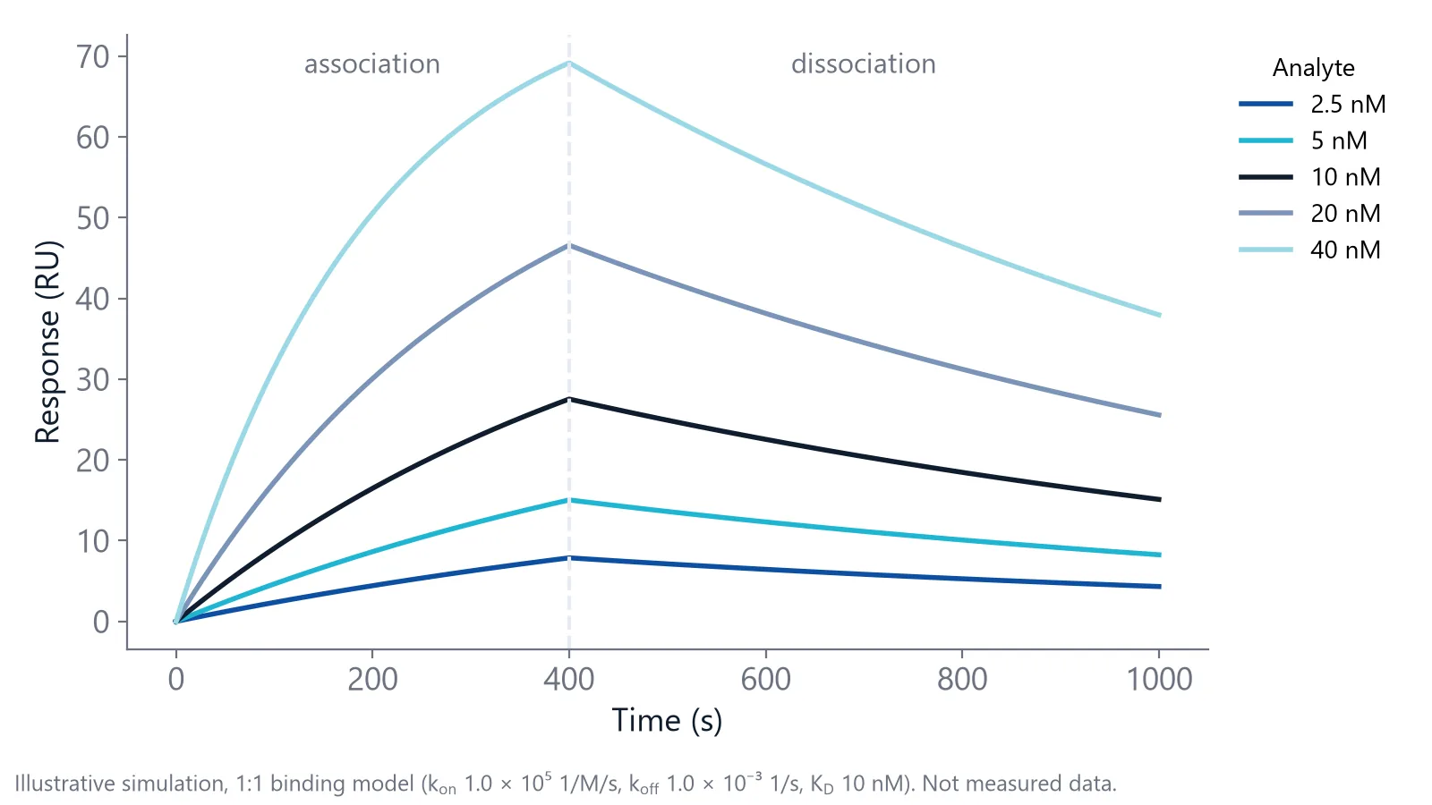
The analyte is injected, binds to the ligand, and the signal rises. How fast it rises depends on the analyte concentration and on the association rate constant, ka (unit 1/M/s, for many protein interactions between 104 and 106). With a long enough injection, the curve flattens into a steady state where binding and unbinding are in balance.
Dissociation
Running buffer replaces the analyte and the complexes fall apart. The speed is set by the dissociation rate constant, kd (unit 1/s). A kd of 10-3 1/s means about 0.1% of the complexes fall apart every second, a half-life of about 11.5 minutes.
Divide kd by ka and you get the dissociation constant, KD, in molar units. In the simulation above, 10-3 divided by 105 gives a KD of 10 nM. A lower KD means tighter binding.
Regeneration
A short pulse of regeneration solution strips the remaining analyte, so the next cycle starts from a clean surface [2]. Low pH or high salt are common choices, as long as the ligand survives them [1]. To check, repeat the same analyte injection several times and compare the binding level and the baseline after each regeneration [3].
The height tells you how much ligand is working
Rmax is the response when every ligand site carries an analyte. It reflects the functional ligand density, which is not the same as the amount you immobilized [1].
Estimate the expected Rmax before you run. Multiply the ligand response by the ratio of analyte to ligand molecular weight, and by the number of binding sites per ligand. Take 1000 RU of a 20 kDa ligand: a 50 kDa analyte can give at most 2500 RU, but a 500 Da compound gives only 25 RU [3]. That is why small molecule binding affinity work depends on a quiet baseline.
A plateau far below the expected Rmax usually means part of the ligand is inactive, or the injection was too short to reach steady state [3].
The plateau also depends on concentration. At an analyte concentration equal to KD, the steady-state response is half of Rmax, and you need at least 10 times KD to reach about 90%. Cover roughly 0.1 to 10 times KD in your concentration series [1].
The shape tells you whether a simple model fits
The shape of the curve matters as much as its height. A 1:1 interaction, where one analyte binds one ligand site with no further steps, rises as a single exponential and decays as a single exponential. That means the curve bends smoothly toward a plateau (or toward zero) at one fixed rate. Other shapes point to a different binding process or to an artifact [4]. Run two checks on your own data:
- Scale the dissociation curves to the same starting height. In a 1:1 interaction they overlap at every concentration, because kd does not depend on concentration.
- Look at the first seconds of the association. A straight rise instead of a curve suggests mass transport limitation: the analyte reaches the surface more slowly than it binds [4].
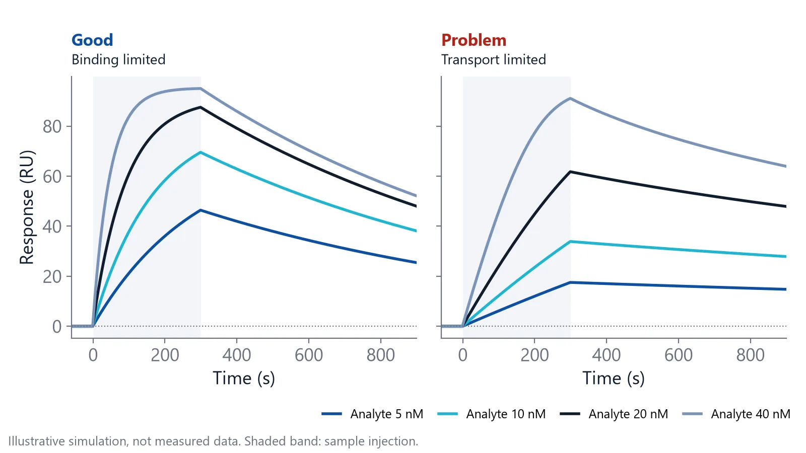
To confirm mass transport limitation, repeat the injection at several flow rates, for example 5, 20, 50 and 100 µL/min, or on a surface with less ligand [4]. If the association gets faster, transport was limiting your curve, not binding.
Give the dissociation enough time. For a slow off-rate, the signal must drop at least 5% from its starting value before kd can be estimated [1].
Why does a sensorgram jump at the start and end of an injection?
Square jumps at the start and end of an injection are usually a bulk shift. The sample buffer has a slightly different refractive index from the running buffer, so the signal steps up when the sample arrives and drops when it leaves [2]. Subtracting a reference surface removes most of it.
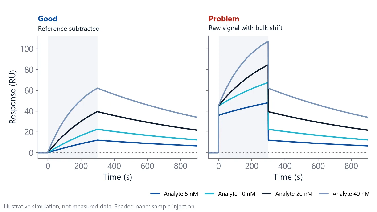
A reference surface carries no ligand, or an inactive one, and sees the same sample. Its signal holds the bulk shift and a little non-specific binding (analyte sticking to the surface rather than to the ligand), so subtracting it removes both [1]. On inQuiQ, one channel is the reference and sits in the same serial flow path as the ligand channels, so it sees the same injection (see the inQuiQ benchtop biosensor).
Then subtract a buffer blank: an injection of matched buffer without analyte, run close in time to your samples, with at least three blanks at the start of the experiment [4]. This second step, called double referencing, removes drift that the reference surface leaves behind [5].
Match the sample buffer to the running buffer to keep the jump small. After referencing, baseline, association and dissociation should connect without steps [4].
Check the baseline before you trust the curve
Drift is a slow slope in the baseline. It usually means the surface is not yet equilibrated, for example right after immobilization, when equilibration can take much longer than a few minutes, sometimes overnight [4]. A change in flow rate can also cause drift that takes 5 to 30 minutes to level out, so run buffer until the baseline is flat and add a few buffer injections before the first sample [4].
On inQuiQ, baseline drift is typically below 0.3 RU/min.
At the end of dissociation, the signal should return to the starting baseline. Serum, plasma and lysates make a residual signal more likely (see binding analysis in serum and plasma).
| What you see | Likely cause | How to check |
|---|---|---|
| Square steps at the start and end of the injection | Bulk shift [2] | See whether the reference channel shows the same steps |
| Slow slope in the baseline | Surface not equilibrated, or a flow rate change [4] | Run buffer until flat, then add buffer injections |
| Straight start of the association | Mass transport limitation [4] | Repeat at a higher flow rate or on a surface with less ligand |
| Signal stays up after dissociation | Non-specific binding to the matrix [1], or a very slow off-rate | See whether the reference channel holds signal too |
| Baseline rises after each cycle | Incomplete regeneration | Repeat identical injections and compare the baseline [3] |
What should a sensorgram look like before you fit it?
A sensorgram is ready to fit when it passes five checks [4]:
- The baseline is flat and stable.
- The buffer jump at injection start and end is tiny.
- After referencing, the phases join smoothly.
- The association starts with a curve, not a straight line.
- The rise and decay follow single exponentials.
Data that pass these checks can often be fitted with a simple 1:1 model across the whole concentration series [6].
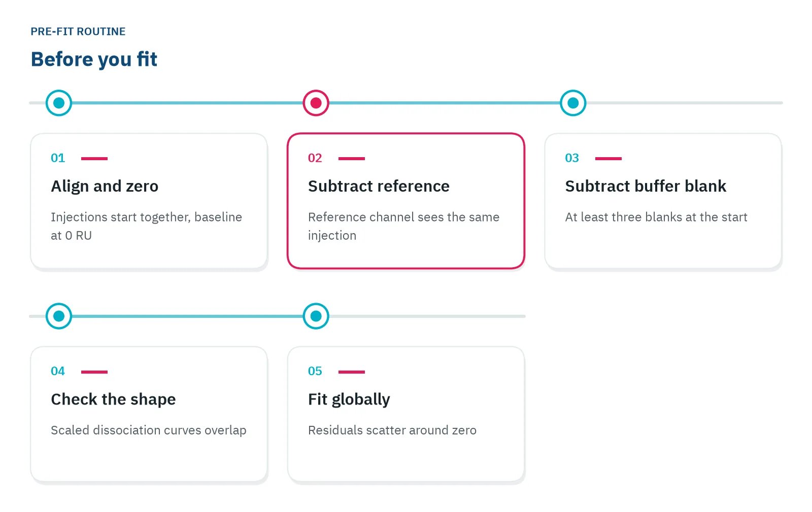
Fit globally: one ka, one kd and one Rmax for all concentrations, so the model must explain every curve at once [3]. Then look at the residuals, the difference between data and fit. They should scatter randomly around zero.
Most artifacts are easier to prevent with a better experiment than to fit away [6].
Questions researchers ask
What does a single-cycle kinetics sensorgram look like?
In single-cycle kinetics you inject increasing analyte concentrations one after another, without regeneration in between, and end with one long dissociation. The sensorgram looks like a staircase that climbs to the highest concentration. You read each step as usual, then fit all steps together in one model.
Do BLI and NES sensorgrams read the same way as SPR sensorgrams?
Yes. Biolayer interferometry (BLI) and Nanophotonic Evanescent field Sensing (NES) also record baseline, association and dissociation over time. The y-axis unit can differ: BLI reports a wavelength shift in nm instead of RU. In BLI the sensor tip moves between wells, so phase changes come from moving the tip, not from switching the flow.
Why does my signal go below baseline after reference subtraction?
A negative signal after subtraction usually means the reference surface gained more than the active surface. Common causes are analyte sticking to the reference, a buffer mismatch that affects the two surfaces differently, or a reference that drifts. Inject the analyte over the reference alone to see which surface behaves differently.
Can I get a KD from a single sensorgram?
You can fit one curve, but the result is fragile, because one concentration cannot show whether the kinetics hold across concentrations. Use a series of at least five concentrations, fit them together as in the global fit above, and repeat one concentration to check reproducibility.
References
- Handbook of Surface Plasmon Resonance. The Royal Society of Chemistry. 2017. doi:10.1039/9781788010283
- Schasfoort RBM. Introduction to Surface Plasmon Resonance. Handbook of Surface Plasmon Resonance. 2017. doi:10.1039/9781788010283-00001
- Real-Time Analysis of Biomolecular Interactions. Springer Japan. 2000. doi:10.1007/978-4-431-66970-8
- Marquart JA. SPRpages – Getting a Feeling for the Curves. Handbook of Surface Plasmon Resonance. 2017. doi:10.1039/9781788010283-00106
- Ditto NT, Eckman J. Treating Raw Data: Software for SPR Applications. Handbook of Surface Plasmon Resonance. 2017. doi:10.1039/9781788010283-00328
- Myszka DG. Improving biosensor analysis. J Mol Recognit. 1999. doi:10.1002/(SICI)1099-1352(199909/10)12:5<279::AID-JMR473>3.0.CO;2-3
Keep reading
 KD vs IC50: how binding affinity and inhibition differKD describes a binding pair, IC50 describes an inhibitor in one assay. Here is how they relate, when you can convert one into the other, and what kinetics add.Label-free 101
 Dissociation constant (KD): what it tells you about bindingWhat a KD value means at the bench, why two binders with the same KD can behave very differently, and the checks that tell you whether a KD is real.Method comparisons
 Biolayer interferometry vs SPR: which method fits your assayBoth methods measure binding label-free and in real time. The sample path, flow over a chip or a tip in a well, decides which one suits your hardest measurement.